Transformers 中的多头注意力机制
位置编码是 Transformer 架构中使用的一个重要组件。位置编码的输出进入 Transformer 架构的第一个子层。该子层是一种多头注意力机制。
多头注意力机制是 Transformer 模型的一个关键特性,可帮助其更有效地处理顺序数据。它允许模型同时查看输入序列的不同部分。
在本章中,我们将探讨多头注意力机制的结构、其优势和 Python 实现。
什么是自注意力机制?
自注意力机制,也称为缩放点积注意力,是基于 Transformer 的模型的重要组成部分。它允许模型关注输入序列中相对于彼此的不同标记。这是通过计算输入值的加权和来实现的。这里的权重基于 token 之间的相似性。
自注意力机制
以下是自注意力机制所涉及的步骤 −
- 创建查询、键和值 − 自注意力机制将输入序列中的每个 token 转换为三个向量,即查询 (Q)、键 (K) 和值 (V)。
- 计算注意力分数 − 接下来,自注意力机制通过对查询 (Q) 和键 (K) 指标进行点积来计算注意力分数。注意力分数显示每个单词对当前正在处理的单词的重要性。
- 应用 Softmax 函数 −现在,在此步骤中,将 softmax 函数应用于这些注意力分数,以将它们转换为概率,从而确保注意力权重总和为 1。
- 值的加权总和 −在最后一步中,为了生成输出,softmax 注意力得分用于计算值向量的加权和。
从数学上讲,自注意力机制可以用以下公式总结:−
$$\mathrm{Self-Attention(Q,K,V) \: = \: softmax \left(\frac{QK^{T}}{\sqrt{d_{k}}}\right)V}$$
什么是多头注意力?
多头注意力扩展了自注意力机制的概念,允许模型同时关注输入序列的不同部分。多头注意力不是运行单个注意力函数,而是并行运行多个自注意力机制或"头"。这种方法使模型能够更好地理解输入序列内的各种关系和依赖关系。
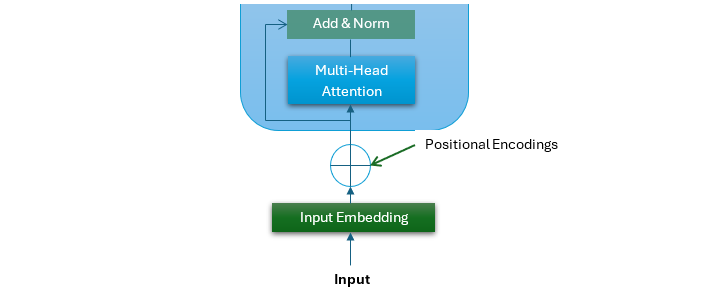
看一下下面的图片,它是原始 Transformer 架构的一部分。它表示多头子层的结构 −
多头注意力的步骤
下面给出了多头注意力的关键步骤 −
- 应用多个头 − 首先,将输入嵌入线性投影到多个集合(每个头一个集合)的查询(Q)、键(K)和值(V)指标中。
- 执行并行自注意力 −接下来,每个头部在其各自的投影上并行执行自我注意机制。
- 连接 − 现在,所有头部的输出都被连接起来。
- 组合信息 − 在最后一步中,所有头部的信息被组合起来。这是通过将连接的输出传递到最终的线性层来完成的。
从数学上讲,多头注意力机制可以通过以下公式总结 −
$$\mathrm{MultiHead(Q,K,V) \: = \: Concat(head_{1}, \: \dotso \: ,head_{h})W^{\circ}}$$
其中每个头的计算方式为 −
$$\mathrm{head_{i}\:=\: Attention(QW_{i}^{Q}, \: KW_{i}^{K}, \: VW_{i}^{V} )\:=\: softmax\left(\frac{QW_{i}^{Q} (KW_{i}^{K})^{T}}{\sqrt{d_{k}}}\right)VW_{i}^{V}}$$
多头注意力机制的优势
增强表征 − 通过同时关注输入序列的不同部分,多头注意力机制使模型能够更好地理解输入序列中的各种关系和依赖关系。
并行处理 − 通过启用并行处理,与 RNN 等顺序模型相比,多头注意力机制可显著提高模型训练效率。
示例
以下 Python 脚本将实现多头注意力机制 −
import numpy as np

class MultiHeadAttention:
   def __init__(self, d_model, num_heads):
      self.d_model = d_model
      self.num_heads = num_heads
      assert d_model % num_heads == 0
      self.depth = d_model // num_heads

      # 初始化查询、键和值的权重矩阵
      self.W_q = np.random.randn(d_model, d_model) * np.sqrt(2 / d_model)
      self.W_k = np.random.randn(d_model, d_model) * np.sqrt(2 / d_model)
      self.W_v = np.random.randn(d_model, d_model) * np.sqrt(2 / d_model)

      # 初始化输出权重矩阵
      self.W_o = np.random.randn(d_model, d_model) * np.sqrt(2 / d_model)

   def split_heads(self, x, batch_size):
      """
      Split the last dimension into (num_heads, depth).
      Transpose the result to shape (batch_size, num_heads, seq_len, depth)
      """
      x = np.reshape(x, (batch_size, -1, self.num_heads, self.depth))
      return np.transpose(x, (0, 2, 1, 3))

   def scaled_dot_product_attention(self, q, k, v):
      """
      Compute scaled dot product attention.
      """
      matmul_qk = np.matmul(q, k)
      scaled_attention_logits = matmul_qk / np.sqrt(self.depth)
      scaled_attention_logits -= np.max(scaled_attention_logits, axis=-1, keepdims=True)
      attention_weights = np.exp(scaled_attention_logits)
      attention_weights /= np.sum(attention_weights, axis=-1, keepdims=True)
      output = np.matmul(attention_weights, v)
      return output, attention_weights

   def call(self, inputs):
        q, k, v = 输入
        batch_size = q.shape[0]

        # 线性变换
        q = np.dot(q, self.W_q)
        k = np.dot(k, self.W_k)
        v = np.dot(v, self.W_v)

        # 分割头部
        q = self.split_heads(q, batch_size)
        k = self.split_heads(k, batch_size)
        v = self.split_heads(v, batch_size)

        # 缩放点积注意力
        tention_output,tention_weights = self.scaled_dot_product_attention(q, k.transpose(0, 1, 3, 2), v)

        # 合并头部
        tention_output = np.transpose(attention_output, (0, 2, 1, 3))
        concat_attention = np.reshape(attention_output, (batch_size, -1, self.d_model))

        # 输出的线性变换
        output = np.dot(concat_attention, self.W_o)

        返回 output,tention_weights

# 示例用法
d_model = 512
num_heads = 8
batch_size = 2
seq_len = 10

# 创建 MultiHeadAttention 实例
multi_head_attn = MultiHeadAttention(d_model, num_heads)

# 示例输入 (batch_size, serial_length, embedding_dim)
Q = np.random.randn(batch_size, seq_len, d_model)
K = np.random.randn(batch_size, seq_len, d_model)
V = np.random.randn(batch_size, seq_len, d_model)

# 执行多头注意
output, attention_weights = multi_head_attn.call([Q, K, V])

print("Input Query (Q):
", Q)
print("Multi-Head Attention Output:
", output)
输出
执行上述脚本后,我们将得到以下输出 −
Input Query (Q):
 [[[ 1.38223113 -0.41160481  1.00938637 ... -0.23466982 -0.20555623  0.80305284]
  [ 0.64676968 -0.83592083  2.45028238 ... -0.1884722  -0.25315478   0.18875416]
  [-0.52094419 -0.03697595 -0.61598294 ...  1.25611974 -0.35473911   0.15091853]
  ...
  [ 1.15939786 -0.5304271  -0.45396363 ...  0.8034571   0.66646109  -1.28586743]
  [ 0.6622964  -0.62871864  0.61371113 ... -0.59802729 -0.66135327  -0.24437055]
  [ 0.83111283 -0.81060387 -0.30858598 ... -0.74773536 -1.3032037   3.06236077]]

 [[-0.88579467 -0.15480352  0.76149486 ... -0.5033709   1.20498808  -0.55297549]
  [-1.11233207  0.7560376  -1.41004173 ... -2.12395203  2.15102493   0.09244935]
  [ 0.33003584  1.67364745 -0.30474183 ...  1.65907682 -0.61370707   0.58373516]
  ...
  [-2.07447136 -1.04964997 -0.15290381 ... -0.19912739 -1.02747937   0.20710549]
  [ 0.38910395 -1.04861089 -1.66583867 ...  0.21530474 -1.45005951   0.04472527]
  [-0.4718725  -0.45374148 -0.59990784 ... -1.9545574   0.11470969 1.03736175]]]

Multi-Head Attention Output:
 [[[ 0.36106079 -2.04297889  0.34937837 ...  0.11306262  0.53263072 -1.32641213]
  [ 1.09494311 -0.56658386  0.24210239 ...  1.1671274  -0.02322074   0.90110388]
  [ 0.45854972 -0.54493138 -0.63421376 ...  1.12479291  0.02585155  -0.08487499]
  ...
  [ 0.18252303 -0.17292067  0.46922657 ... -0.41311278 -1.17954406  -0.17005412]
  [-0.7849032  -2.12371221 -0.80403028 ... -2.35884088  0.15292393  -0.05569091]
  [ 1.07844261  0.18249226  0.81735183 ...  1.16346645 -1.71611237 -1.09860234]]

 [[ 0.58842816 -0.04493786 -1.72007093 ... -2.37506208 -1.83098896   2.84016717]
  [ 0.36608434  0.11709812  0.79108595 ... -1.6308595  -0.96052828   0.40893208]
  [-1.42113667  0.67459219 -0.8731377  ... -1.47390056 -0.42947079   1.04828361]
  ...
  [ 1.14151388 -1.5437165  -1.23405718 ...  0.29237056  0.56595327  -0.19385628]
  [-2.33028535  0.7245296   1.01725021 ... -0.9380485  -1.78988485   0.9938851 ]
  [-0.88115094  3.03051907  0.39447342 ... -1.89168756  0.94973626   0.61657539]
]]
结论
多头注意力子层是 Transformer 架构的关键组件。它允许模型同时查看输入序列的不同部分,从而帮助模型更有效地处理顺序数据。
在本章中,我们全面概述了多头注意力机制、其优势以及如何使用 Python 实现它。