Floyd Warshall Algorithm

The Floyd-Warshall algorithm is a graph algorithm that is deployed to find the shortest path between all the vertices present in a weighted graph. This algorithm is different from other shortest path algorithms; to describe it simply, this algorithm uses each vertex in the graph as a pivot to check if it provides the shortest way to travel from one point to another.
Floyd-Warshall algorithm works on both directed and undirected weighted graphs unless these graphs do not contain any negative cycles in them. By negative cycles, it is meant that the sum of all the edges in the graph must not lead to a negative number.
Since, the algorithm deals with overlapping sub-problems – the path found by the vertices acting as pivot are stored for solving the next steps – it uses the dynamic programming approach.
Floyd-Warshall algorithm is one of the methods in All-pairs shortest path algorithms and it is solved using the Adjacency Matrix representation of graphs.
Floyd-Warshall Algorithm
Consider a graph, G = {V, E} where V is the set of all vertices present in the graph and E is the set of all the edges in the graph. The graph, G, is represented in the form of an adjacency matrix, A, that contains all the weights of every edge connecting two vertices.
Algorithm
Step 1 − Construct an adjacency matrix A with all the costs of edges present in the graph. If there is no path between two vertices, mark the value as ∞.
Step 2 − Derive another adjacency matrix A1 from A keeping the first row and first column of the original adjacency matrix intact in A1. And for the remaining values, say A1[i,j], if A[i,j]>A[i,k]+A[k,j] then replace A1[i,j] with A[i,k]+A[k,j]. Otherwise, do not change the values. Here, in this step, k = 1 (first vertex acting as pivot).
Step 3 − Repeat Step 2 for all the vertices in the graph by changing the k value for every pivot vertex until the final matrix is achieved.
Step 4 − The final adjacency matrix obtained is the final solution with all the shortest paths.
Pseudocode
Floyd-Warshall(w, n){ // w: weights, n: number of vertices
   for i = 1 to n do // initialize, D (0) = [wij]
      for j = 1 to n do{
         d[i, j] = w[i, j];
      }
      for k = 1 to n do // Compute D (k) from D (k-1)
         for i = 1 to n do
            for j = 1 to n do
               if (d[i, k] + d[k, j] < d[i, j]){
                  d[i, j] = d[i, k] + d[k, j];
               }
      return d[1..n, 1..n];
}
Example
Consider the following directed weighted graph G = {V, E}. Find the shortest paths between all the vertices of the graphs using the Floyd-Warshall algorithm.
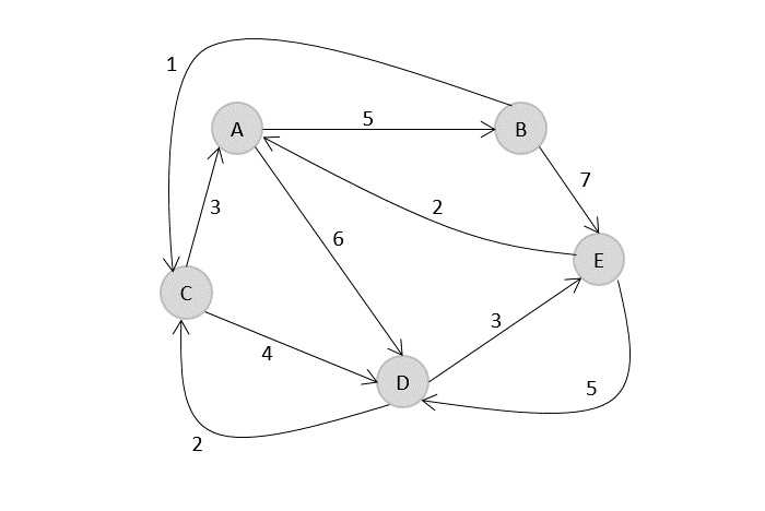
Solution
Step 1
Construct an adjacency matrix A with all the distances as values.
$$A=\begin{matrix} 0 & 5& \infty & 6& \infty \ \infty & 0& 1& \infty& 7\ 3 & \infty& 0& 4& \infty\ \infty & \infty& 2& 0& 3\ 2& \infty& \infty& 5& 0\ \end{matrix}$$
Step 2
Considering the above adjacency matrix as the input, derive another matrix A0 by keeping only first rows and columns intact. Take k = 1, and replace all the other values by A[i,k]+A[k,j].
$$A=\begin{matrix} 0 & 5& \infty & 6& \infty \ \infty & & & & \ 3& & & & \ \infty& & & & \ 2& & & & \ \end{matrix}$$
$$A_{1}=\begin{matrix} 0 & 5& \infty & 6& \infty \ \infty & 0& 1& \infty& 7\ 3 & 8& 0& 4& \infty\ \infty & \infty& 2& 0& 3\ 2& 7& \infty& 5& 0\ \end{matrix}$$
Step 3
Considering the above adjacency matrix as the input, derive another matrix A0 by keeping only first rows and columns intact. Take k = 1, and replace all the other values by A[i,k]+A[k,j].
$$A_{2}=\begin{matrix} & 5& & & \ \infty & 0& 1& \infty& 7\ & 8& & & \ & \infty& & & \ & 7& & & \ \end{matrix}$$
$$A_{2}=\begin{matrix} 0 & 5& 6& 6& 12 \ \infty & 0& 1& \infty& 7\ 3 & 8& 0& 4& 15\ \infty & \infty& 2& 0& 3\ 2 & 7& 8& 5& 0 \ \end{matrix}$$
Step 4
Considering the above adjacency matrix as the input, derive another matrix A0 by keeping only first rows and columns intact. Take k = 1, and replace all the other values by A[i,k]+A[k,j].
$$A_{3}=\begin{matrix} & & 6& & \ & & 1& & \ 3 & 8& 0& 4& 15\ & & 2& & \ & & 8& & \ \end{matrix}$$
$$A_{3}=\begin{matrix} 0 & 5& 6& 6& 12 \ 4 & 0& 1& 5& 7\ 3 & 8& 0& 4& 15\ 5 & 10& 2& 0& 3\ 2 & 7& 8& 5& 0 \ \end{matrix}$$
Step 5
Considering the above adjacency matrix as the input, derive another matrix A0 by keeping only first rows and columns intact. Take k = 1, and replace all the other values by A[i,k]+A[k,j].
$$A_{4}=\begin{matrix} & & & 6& \ & & & 5& \ & & & 4& \ 5 & 10& 2& 0& 3\ & & & 5& \ \end{matrix}$$
$$A_{4}=\begin{matrix} 0 & 5& 6& 6& 9 \ 4 & 0& 1& 5& 7\ 3 & 8& 0& 4& 7\ 5 & 10& 2& 0& 3\ 2 & 7& 7& 5& 0 \ \end{matrix}$$
Step 6
Considering the above adjacency matrix as the input, derive another matrix A0 by keeping only first rows and columns intact. Take k = 1, and replace all the other values by A[i,k]+A[k,j].
$$A_{5}=\begin{matrix} & & & & 9 \ & & & & 7\ & & & & 7\ & & & & 3\ 2 & 7& 7& 5& 0 \ \end{matrix}$$
$$A_{5}=\begin{matrix} 0 & 5& 6& 6& 9 \ 4 & 0& 1& 5& 7\ 3 & 8& 0& 4& 7\ 5 & 10& 2& 0& 3\ 2 & 7& 7& 5& 0 \ \end{matrix}$$
Analysis
From the pseudocode above, the Floyd-Warshall algorithm operates using three for loops to find the shortest distance between all pairs of vertices within a graph. Therefore, the time complexity of the Floyd-Warshall algorithm is O(n3), where ‘n’ is the number of vertices in the graph. The space complexity of the algorithm is O(n2).
Implementation
Following is the implementation of Floyd Warshall Algorithm to find the shortest path in a graph using cost adjacency matrix -
#include <stdio.h>
void floyds(int b[3][3]) {
   int i, j, k;
   for (k = 0; k < 3; k++) {
      for (i = 0; i < 3; i++) {
         for (j = 0; j < 3; j++) {
            if ((b[i][k] * b[k][j] != 0) && (i != j)) {
               if ((b[i][k] + b[k][j] < b[i][j]) || (b[i][j] == 0)) {
                  b[i][j] = b[i][k] + b[k][j];
               }
            }
         }
      }
   }
   for (i = 0; i < 3; i++) {
      printf("Minimum Cost With Respect to Node: %d
", i);
      for (j = 0; j < 3; j++) {
         printf("%d	", b[i][j]);
      }
   }
}

int main() {
   int b[3][3] = {0};
   b[0][1] = 10;
   b[1][2] = 15;
   b[2][0] = 12;
   floyds(b);
   return 0;
}
Output
Minimum Cost With Respect to Node: 0
0	10	25
Minimum Cost With Respect to Node: 1
27	0	15
Minimum Cost With Respect to Node: 2
12	22	0
#include <iostream>
using namespace std;
void floyds(int b[][3]){
   int i, j, k;
   for (k = 0; k < 3; k++) {
      for (i = 0; i < 3; i++) {
         for (j = 0; j < 3; j++) {
            if ((b[i][k] * b[k][j] != 0) && (i != j)) {
               if ((b[i][k] + b[k][j] < b[i][j]) || (b[i][j] == 0)) {
                  b[i][j] = b[i][k] + b[k][j];
               }
            }
         }
      }
   }
   for (i = 0; i < 3; i++) {
      cout<<"Minimum Cost With Respect to Node:"<<i<<endl;
      for (j = 0; j < 3; j++) {
         cout<<b[i][j]<<"	";
      }
   }
}
int main(){
   int b[3][3];
   for (int i = 0; i < 3; i++) {
      for (int j = 0; j < 3; j++) {
         b[i][j] = 0;
      }
   }
   b[0][1] = 10;
   b[1][2] = 15;
   b[2][0] = 12;
   floyds(b);
   return 0;
}
Output
Minimum Cost With Respect to Node:0
0  10  25
Minimum Cost With Respect to Node:1
27  0  15
Minimum Cost With Respect to Node:2
12  22  0
import java.util.Arrays;
public class Main {
   public static void floyds(int[][] b) {
      int i, j, k;
      for (k = 0; k < 3; k++) {
         for (i = 0; i < 3; i++) {
            for (j = 0; j < 3; j++) {
               if ((b[i][k] * b[k][j] != 0) && (i != j)) {
                  if ((b[i][k] + b[k][j] < b[i][j]) || (b[i][j] == 0)) {
                     b[i][j] = b[i][k] + b[k][j];
                  }
               }
            }
         }
      }
      for (i = 0; i < 3; i++) {
         System.out.println("Minimum Cost With Respect to Node:" + i);
         for (j = 0; j < 3; j++) {
            System.out.print(b[i][j] + "	");
         }
      }
   }
   public static void main(String[] args) {
      int[][] b = new int[3][3];
      for (int i = 0; i < 3; i++) {
         Arrays.fill(b[i], 0);
      }
      b[0][1] = 10;
      b[1][2] = 15;
      b[2][0] = 12;
      floyds(b);
   }
}
Output
Minimum Cost With Respect to Node:0
0  10  25
Minimum Cost With Respect to Node:1
27  0  15
Minimum Cost With Respect to Node:2
12  22  0
import numpy as np
def floyds(b):
    for k in range(3):
        for i in range(3):
            for j in range(3):
                if (b[i][k] * b[k][j] != 0) and (i != j):
                    if (b[i][k] + b[k][j] < b[i][j]) or (b[i][j] == 0):
                        b[i][j] = b[i][k] + b[k][j]
    for i in range(3):
        print("Minimum Cost With Respect to Node:", i)
        for j in range(3):
            print(b[i][j], end="	")
b = np.zeros((3, 3), dtype=int)
b[0][1] = 10
b[1][2] = 15
b[2][0] = 12
#calling the method
floyds(b)
Output
Minimum Cost With Respect to Node: 0
0	10	25
Minimum Cost With Respect to Node: 1
27	0	15
Minimum Cost With Respect to Node: 2
12	22	0