Data Structures - Asymptotic Analysis

Asymptotic Analysis
Asymptotic analysis of an algorithm refers to defining the mathematical foundation/framing of its run-time performance. Using asymptotic analysis, we can very well conclude the best case, average case, and worst case scenario of an algorithm.
Asymptotic analysis is input bound i.e., if there's no input to the algorithm, it is concluded to work in a constant time. Other than the "input" all other factors are considered constant.
Asymptotic analysis refers to computing the running time of any operation in mathematical units of computation. For example, the running time of one operation is computed as f(n) and may be for another operation it is computed as g(n2). This means the first operation running time will increase linearly with the increase in n and the running time of the second operation will increase exponentially when n increases. Similarly, the running time of both operations will be nearly the same if n is significantly small.
Usually, the time required by an algorithm falls under three types −
Best Case − Minimum time required for program execution.
Average Case − Average time required for program execution.
Worst Case − Maximum time required for program execution.
Asymptotic Notations
Execution time of an algorithm depends on the instruction set, processor speed, disk I/O speed, etc. Hence, we estimate the efficiency of an algorithm asymptotically.
Time function of an algorithm is represented by T(n), where n is the input size.
Different types of asymptotic notations are used to represent the complexity of an algorithm. Following asymptotic notations are used to calculate the running time complexity of an algorithm.
O − Big Oh Notation
Ω − Big omega Notation
θ − Big theta Notation
o − Little Oh Notation
ω − Little omega Notation
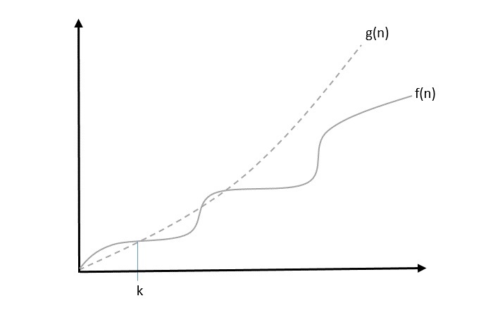
Big Oh, O: Asymptotic Upper Bound
The notation Ο(n) is the formal way to express the upper bound of an algorithm's running time. is the most commonly used notation. It measures the worst case time complexity or the longest amount of time an algorithm can possibly take to complete.
A function f(n) can be represented is the order of g(n) that is O(g(n)), if there exists a value of positive integer n as n0 and a positive constant c such that −
$f(n)\leqslant c.g(n)$ for $n > n_{0}$ in all case
Hence, function g(n) is an upper bound for function f(n), as g(n) grows faster than f(n).
Example
Let us consider a given function, $f(n) = 4.n^3 + 10.n^2 + 5.n + 1$
Considering $g(n) = n^3$,
$f(n)\leqslant 5.g(n)$ for all the values of $n > 2$
Hence, the complexity of f(n) can be represented as $O(g(n))$, i.e. $O(n^3)$
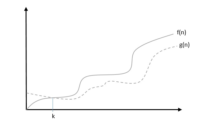
Big Omega, Ω: Asymptotic Lower Bound
The notation Ω(n) is the formal way to express the lower bound of an algorithm's running time. It measures the best case time complexity or the best amount of time an algorithm can possibly take to complete.
We say that $f(n) = \Omega (g(n))$ when there exists constant c that $f(n)\geqslant c.g(n)$ for all sufficiently large value of n. Here n is a positive integer. It means function g is a lower bound for function f ; after a certain value of n, f will never go below g.
Example
Let us consider a given function, $f(n) = 4.n^3 + 10.n^2 + 5.n + 1$.
Considering $g(n) = n^3$, $f(n)\geqslant 4.g(n)$ for all the values of $n > 0$.
Hence, the complexity of f(n) can be represented as $\Omega (g(n))$, i.e. $\Omega (n^3)$
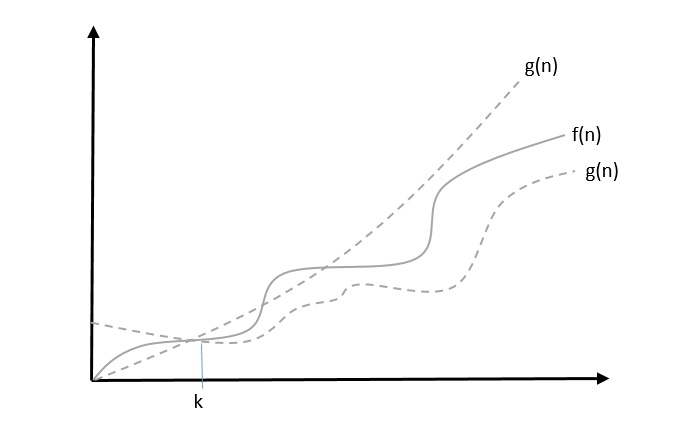
Theta, θ: Asymptotic Tight Bound
The notation θ(n) is the formal way to express both the lower bound and the upper bound of an algorithm's running time. Some may confuse the theta notation as the average case time complexity; while big theta notation could be almost accurately used to describe the average case, other notations could be used as well.
We say that $f(n) = heta(g(n))$ when there exist constants c1 and c2 that $c_{1}.g(n) \leqslant f(n) \leqslant c_{2}.g(n)$ for all sufficiently large value of n. Here n is a positive integer.
This means function g is a tight bound for function f.
Example
Let us consider a given function, $f(n) = 4.n^3 + 10.n^2 + 5.n + 1$
Considering $g(n) = n^3$, $4.g(n) \leqslant f(n) \leqslant 5.g(n)$ for all the large values of n.
Hence, the complexity of f(n) can be represented as $ heta (g(n))$, i.e. $ heta (n^3)$.
Little Oh, o
The asymptotic upper bound provided by O-notation may or may not be asymptotically tight. The bound $2.n^2 = O(n^2)$ is asymptotically tight, but the bound $2.n = O(n^2)$ is not.
We use o-notation to denote an upper bound that is not asymptotically tight.
We formally define o(g(n)) (little-oh of g of n) as the set f(n) = o(g(n)) for any positive constant $c > 0$ and there exists a value $n_{0} > 0$, such that $0 \leqslant f(n) \leqslant c.g(n)$.
Intuitively, in the o-notation, the function f(n) becomes insignificant relative to g(n) as n approaches infinity; that is,
$$\lim_{n ightarrow \infty}\left(\frac{f(n)}{g(n)} ight) = 0$$
Example
Let us consider the same function, $f(n) = 4.n^3 + 10.n^2 + 5.n + 1$
Considering $g(n) = n^{4}$,
$$\lim_{n ightarrow \infty}\left(\frac{4.n^3 + 10.n^2 + 5.n + 1}{n^4} ight) = 0$$
Hence, the complexity of f(n) can be represented as $o(g(n))$, i.e. $o(n^4)$.
Little Omega, ω
We use ω-notation to denote a lower bound that is not asymptotically tight. Formally, however, we define ω(g(n)) (little-omega of g of n) as the set f(n) = ω(g(n)) for any positive constant C > 0 and there exists a value $n_{0} > 0$, such that $0 \leqslant c.g(n) < f(n)$.
For example, $\frac{n^2}{2} = \omega (n)$, but $\frac{n^2}{2} eq \omega (n^2)$. The relation $f(n) = \omega (g(n))$ implies that the following limit exists
$$\lim_{n ightarrow \infty}\left(\frac{f(n)}{g(n)} ight) = \infty$$
That is, f(n) becomes arbitrarily large relative to g(n) as n approaches infinity.
Example
Let us consider same function, $f(n) = 4.n^3 + 10.n^2 + 5.n + 1$
Considering $g(n) = n^2$,
$$\lim_{n ightarrow \infty}\left(\frac{4.n^3 + 10.n^2 + 5.n + 1}{n^2} ight) = \infty$$
Hence, the complexity of f(n) can be represented as $o(g(n))$, i.e. $\omega (n^2)$.
Common Asymptotic Notations
Following is a list of some common asymptotic notations −
| constant | − | O(1) |
| logarithmic | − | O(log n) |
| linear | − | O(n) |
| n log n | − | O(n log n) |
| quadratic | − | O(n2) |
| cubic | − | O(n3) |
| polynomial | − | nO(1) |
| exponential | − | 2O(n) |
Apriori and Apostiari Analysis
Apriori analysis means, analysis is performed prior to running it on a specific system. This analysis is a stage where a function is defined using some theoretical model. Hence, we determine the time and space complexity of an algorithm by just looking at the algorithm rather than running it on a particular system with a different memory, processor, and compiler.
Apostiari analysis of an algorithm means we perform analysis of an algorithm only after running it on a system. It directly depends on the system and changes from system to system.
In an industry, we cannot perform Apostiari analysis as the software is generally made for an anonymous user, which runs it on a system different from those present in the industry.
In Apriori, it is the reason that we use asymptotic notations to determine time and space complexity as they change from computer to computer; however, asymptotically they are the same.