LightGBM - 在 Python 中实现
在本章中,我们将了解在 Python 中开发 LightGBM 模型的步骤。我们将使用 Scikit-learn 的 load_breast_cancer 数据集构建二元分类模型。步骤如下:加载数据、为 LightGBM 准备数据、建立参数、训练模型、进行预测并评估结果。
LightGBM 的实现
因此,让我们使用 Python − 创建一个基本模型
1. 加载数据集
首先,我们使用 Scikit-learn 的 load_breast_cancer 方法加载数据集。该数据集包含乳腺癌分类的特征和标签。
from sklearn.datasets import load_breast_cancer

# 加载数据集
data = load_breast_cancer()
X = data.data
y = data.target
2. 分割数据
使用 Scikit-learn 的 train_test_split 方法将数据集分割为训练集和测试集。这样我们就可以在一组数据上训练模型,然后在另一组数据上评估其性能。
from sklearn.model_selection import train_test_split

# 分割数据
X_train, X_test, y_train, y_test = train_test_split(X, y, test_size=0.2, random_state=42)
3. 为 LightGBM 准备数据
将训练和测试数据转换为 LightGBM 数据集格式。此步骤优化了LightGBM训练算法的数据格式。
import lightgbm as lgb

# 将数据转换为LightGBM数据集格式
train_data = lgb.Dataset(X_train, label=y_train)
test_data = lgb.Dataset(X_test, label=y_test, reference=train_data)
4. 定义参数
设置LightGBM模型的参数。这些参数包括目标函数、评估指标、学习率、叶子计数和最大树深度。
params = {
    'objective': 'binary',
    'metric': 'binary_logloss',
    'boosting_type': 'gbdt',
    'learning_rate': 0.1,
    # 从 31 增加
    'num_leaves': 63,
    # 设置为正值以限制深度
    'max_depth': 10
}
5. 训练模型
使用训练数据训练 LightGBM 模型。为了防止过度拟合,我们使用提前停止,这意味着当验证集上没有看到任何进展时训练结束。
# 使用提前停止训练模型
lgb_model = lgb.train(
    params,
    train_data,
    num_boost_round=100,
    valid_sets=[test_data],
    # 使用回调进行提前停止
    callbacks=[lgb.early_stopping(stopping_rounds=10)]
)
输出
以下是上述步骤的结果 −
[LightGBM] [Info] Number of positive: 286, number of negative: 169
[LightGBM] [Info] Auto-choosing col-wise multi-threading, the overhead of testing was 0.000734 seconds.
You can set `force_col_wise=true` to remove the overhead.
[LightGBM] [Info] Total Bins 4548
[LightGBM] [Info] Number of data points in the train set: 455, number of used features: 30
[LightGBM] [Info] [binary:BoostFromScore]: pavg=0.628571 -> initscore=0.526093
[LightGBM] [Info] Start training from score 0.526093
[LightGBM] [Warning] No further splits with positive gain, best gain: -inf
[LightGBM] [Warning] No further splits with positive gain, best gain: -inf
6. 进行预测
使用训练模型预测测试数据。我们将概率返回为二进制结果。
# 在测试集上进行预测
y_pred = lgb_model.predict(X_test)
y_pred_binary = [1 if x > 0.5 else 0 for x in y_pred]
7. 评估模型
计算测试集的准确度分数以评估模型的性能。这使我们能够了解模型在使用之前未见过的数据时的表现。
from sklearn.metrics import accuracy_score

# 评估模型
accuracy = accuracy_score(y_test, y_pred_binary)
print(f"Accuracy: {accuracy:.2f}")
输出
这是上述模型的准确率 −
准确率:0.96
LightGBM 模型的探索性数据分析 (EDA)
在训练和测试 LightGBM 模型之前必须进行探索性数据分析 (EDA),以便了解数据集、识别模式并为建模做好准备。 EDA 涉及检查数据集的结构、分布、相关性和潜在问题。
以下是使用 EDA 处理 load_breast_cancer 数据集的步骤 −
1. 加载和检查数据集
首先,我们必须加载数据集并检查其基本结构,如样本数量、特征和目标变量。
import pandas as pd
from sklearn.datasets import load_breast_cancer

# 加载数据集
data = load_breast_cancer()
df = pd.DataFrame(data.data, columns=data.feature_names)
df['target'] = data.target

# 检查数据集
print(df.head())
print(df.info())
print(df.describe())
输出
这将导致以下结果:
   mean radius  mean texture  mean perimeter  mean area  mean smoothness  \
0        17.99         10.38          122.80     1001.0          0.11840
1        20.57         17.77          132.90     1326.0          0.08474
2        19.69         21.25          130.00     1203.0          0.10960
3        11.42         20.38           77.58      386.1          0.14250
4        20.29         14.34          135.10     1297.0          0.10030

   mean compactness  mean concavity  mean concave points  mean symmetry  \
0           0.27760          0.3001              0.14710         0.2419
1           0.07864          0.0869              0.07017         0.1812
2           0.15990          0.1974              0.12790         0.2069
3           0.28390          0.2414              0.10520         0.2597
4           0.13280          0.1980              0.10430         0.1809

   mean fractal dimension  ...  worst texture  worst perimeter  worst area  \
0                 0.07871  ...          17.33           184.60      2019.0
1                 0.05667  ...          23.41           158.80      1956.0
2                 0.05999  ...          25.53           152.50      1709.0
3                 0.09744  ...          26.50            98.87       567.7
4                 0.05883  ...          16.67           152.20      1575.0

   worst smoothness  worst compactness  worst concavity  worst concave points  \
0            0.1622             0.6656           0.7119                0.2654
1            0.1238             0.1866           0.2416                0.1860
2            0.1444             0.4245           0.4504                0.2430
3            0.2098             0.8663           0.6869                0.2575
4            0.1374             0.2050           0.4000                0.1625

   worst symmetry  worst fractal dimension  target
0          0.4601                  0.11890       0
1          0.2750                  0.08902       0
2          0.3613                  0.08758       0
3          0.6638                  0.17300       0
4          0.2364                  0.07678       0
2. 检查缺失值
现在让我们看看数据集中是否有任何缺失值。
# 检查缺失值
print(df.isnull().sum())
输出
这将生成以下结果:
mean radius                0
mean texture               0
mean perimeter             0
mean area                  0
mean smoothness            0
mean compactness           0
mean concavity             0
mean concave points        0
mean symmetry              0
mean fractal dimension     0
radius error               0
texture error              0
perimeter error            0
area error                 0
smoothness error           0
compactness error          0
concavity error            0
concave points error       0
symmetry error             0
fractal dimension error    0
worst radius               0
worst texture              0
worst perimeter            0
worst area                 0
worst smoothness           0
worst compactness          0
worst concavity            0
worst concave points       0
worst symmetry             0
worst fractal dimension    0
target                     0
dtype: int64
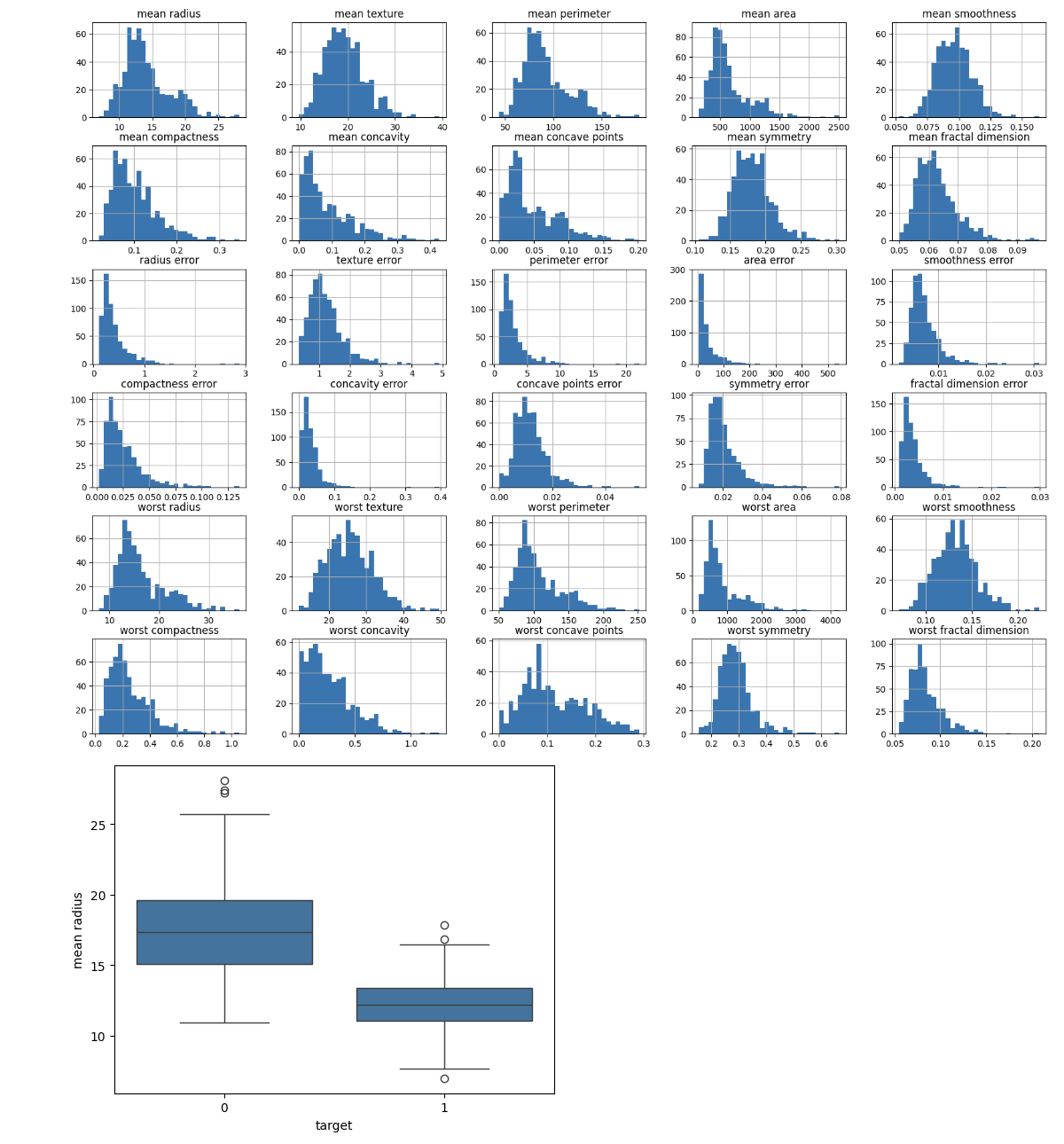
3. 特征分布
确定每个特征的分布。要了解有关特征值的范围和分布的更多信息,请使用直方图、箱线图或其他可视化效果。
import matplotlib.pyplot as plt
import seaborn as sns

# 为每个特征绘制直方图
df.iloc[:, :-1].hist(bins=30, figsize=(20, 15))
plt.show()

# 选定特征的箱线图
sns.boxplot(x='target', y='mean radius', data=df)
plt.show()
输出
这将创建以下结果:
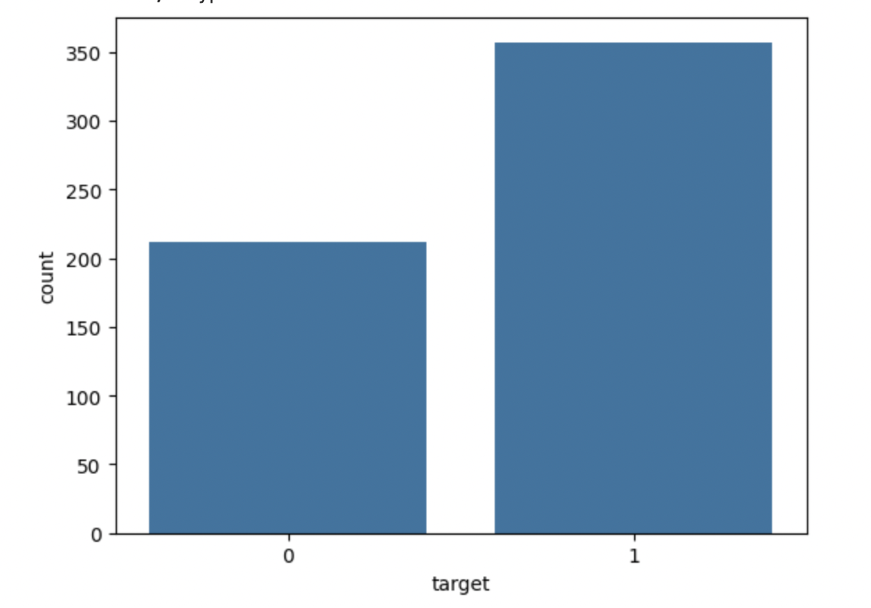
4.分析类别分布
检查目标变量的分布以找到类别平衡。这将允许您识别数据集是否不平衡。
# 类别分布
print(df['target'].value_counts())
sns.countplot(x='target', data=df)
plt.show()
输出
这将显示以下输出 −
target
1    357
0    212
Name: count, dtype: int64
总结
按照这些步骤,您可以创建并测试用于 Python 分类问题的 LightGBM 模型。可以根据需要调整参数和准备步骤,针对不同的数据集和问题修改此技术。