Caffe2 - 使用预训练模型进行图像分类
在本课中,您将学习使用预训练模型来检测给定图像中的对象。您将使用 squeezenet 预训练模块,该模块可以高精度地检测和分类给定图像中的对象。
打开一个新的 Juypter 笔记本 并按照步骤开发此图像分类应用程序。
导入库
首先,我们使用以下代码导入所需的包 −
from caffe2.proto import caffe2_pb2
from caffe2.python import core, working, models
import numpy as np
import skimage.io
import skimage.transform
from matplotlib import pyplot
import os
import urllib.request as urllib2
import operator
接下来,我们设置一些 变量 −
INPUT_IMAGE_SIZE = 227
mean = 128
用于训练的图像显然大小各异。所有这些图像都必须转换为固定大小才能进行准确训练。同样,测试图像和您想要在生产环境中预测的图像也必须转换为与训练期间使用的大小相同的大小。因此,我们创建了一个名为INPUT_IMAGE_SIZE的变量,其值为227。因此,在分类器中使用它之前,我们将所有图像转换为227x227的大小。
我们还声明了一个名为mean的变量,其值为128,稍后用于改进分类结果。
接下来,我们将开发两个用于处理图像的函数。
图像处理
图像处理包括两个步骤。第一个是调整图像大小,第二个是居中裁剪图像。对于这两个步骤,我们将编写两个函数用于调整大小和裁剪。
图像调整大小
首先,我们将编写一个调整图像大小的函数。如前所述,我们将图像大小调整为<b>227x227。因此,让我们将函数resize定义如下 −
def resize(img, input_height, input_width):
我们通过将宽度除以高度来获得图像的纵横比。
original_aspect = img.shape[1]/float(img.shape[0])
如果纵横比大于 1,则表示图像较宽,也就是说处于横向模式。我们现在使用以下代码调整图像高度并返回调整大小后的图像 −
if(original_aspect>1):
   new_height = int(original_aspect * input_height)
   return skimage.transform.resize(img, (input_width,
   new_height), mode='constant', anti_aliasing=True, anti_aliasing_sigma=None)
如果宽高比小于 1,则表示纵向模式。我们现在使用以下代码调整宽度 −
if(original_aspect<1):
   new_width = int(input_width/original_aspect)
   return skimage.transform.resize(img, (new_width,
   input_height), mode='constant', anti_aliasing=True, anti_aliasing_sigma=None)
如果纵横比等于 1,我们不进行任何高度/宽度调整。
if(original_aspect == 1):
    return skimage.transform.resize(img, (input_width,
    input_height), mode='constant', anti_aliasing=True, anti_aliasing_sigma=None)
下面给出了完整的函数代码,供您快速参考 −
def resize(img, input_height, input_width):
   original_aspect = img.shape[1]/float(img.shape[0])
   if(original_aspect>1):
      new_height = int(original_aspect * input_height)
      return skimage.transform.resize(img, (input_width,
	   new_height), mode='constant', anti_aliasing=True, anti_aliasing_sigma=None)
   if(original_aspect<1):
         new_width = int(input_width/original_aspect)
         return skimage.transform.resize(img, (new_width,
         input_height), mode='constant', anti_aliasing=True, anti_aliasing_sigma=None)
   if(original_aspect == 1):
         return skimage.transform.resize(img, (input_width,
         input_height), mode='constant', anti_aliasing=True, anti_aliasing_sigma=None)
现在我们将编写一个函数来裁剪图像的中心。
图像裁剪
我们声明 crop_image 函数如下 −
def crop_image(img,cropx,cropy):
我们使用以下语句提取图像的尺寸 −
y,x,c = img.shape
我们使用以下两行代码为图像创建一个新的起点 −
startx = x//2-(cropx//2)
starty = y//2-(cropy//2)
最后,我们通过创建具有新尺寸的图像对象来返回裁剪后的图像 −
return img[starty:starty+cropy,startx:startx+cropx]
下面给出了完整的函数代码,供您快速参考 −
def crop_image(img,cropx,cropy):
   y,x,c = img.shape
   startx = x//2-(cropx//2)
   starty = y//2-(cropy//2)
   return img[starty:starty+cropy,startx:startx+cropx]
现在,我们将编写代码来测试这些功能。
处理图像
首先,将图像文件复制到项目目录中的 images 子文件夹中。tree.jpg 文件已复制到项目中。以下 Python 代码加载图像并将其显示在控制台上 −
img = skimage.img_as_float(skimage.io.imread("images/tree.jpg")).astype(np.float32)
print("Original Image Shape: " , img.shape)
pyplot.figure()
pyplot.imshow(img)
pyplot.title('Original image')
输出如下 −
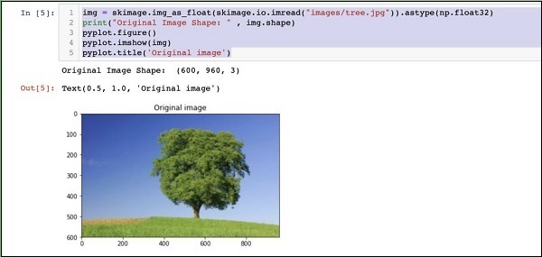
请注意,原始图像的大小为 600 x 960。我们需要将其调整为我们的规格 227 x 227。调用我们之前定义的 resize 函数即可完成此工作。
img = resize(img, INPUT_IMAGE_SIZE, INPUT_IMAGE_SIZE)
print("调整大小后的图像形状: " , img.shape)
pyplot.figure()
pyplot.imshow(img)
pyplot.title('调整大小后的图像')
输出如下所示 −
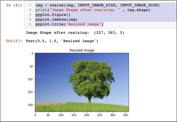
请注意,现在图像大小为 227 x 363。我们需要将其裁剪为 227 x 227,以便最终提供给我们的算法。为此,我们调用了先前定义的裁剪函数。
img = crop_image(img, INPUT_IMAGE_SIZE, INPUT_IMAGE_SIZE)
print("裁剪后的图像形状: " , img.shape)
pyplot.figure()
pyplot.imshow(img)
pyplot.title('Center Cropped')
下面提到的是代码 − 的输出
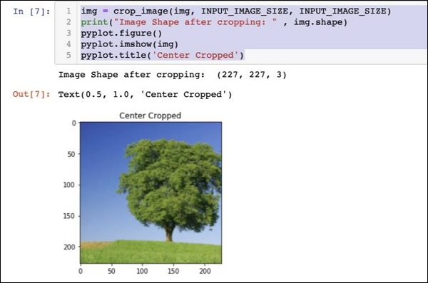
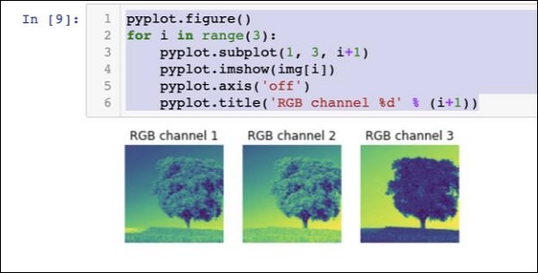
此时,图像尺寸为 227 x 227,可以进行进一步处理。我们现在交换图像轴,将三种颜色提取到三个不同的区域中。
img = img.swapaxes(1, 2).swapaxes(0, 1)
print("CHW Image Shape: " , img.shape)
下面给出的是输出 −
CHW Image Shape: (3, 227, 227)
请注意,最后一个轴现在已成为数组中的第一个维度。我们现在将使用以下代码绘制三个通道 −
pyplot.figure()
for i in range(3):
   pyplot.subplot(1, 3, i+1)
   pyplot.imshow(img[i])
   pyplot.axis('off')
   pyplot.title('RGB channel %d' % (i+1))
输出结果如下所示 −
最后,我们对图像进行一些额外的处理,例如将 Red Green Blue 转换为 Blue Green Red (RGB to BGR),删除平均值以获得更好的结果,并使用以下三行代码添加批量大小轴 −
# convert RGB --> BGR
img = img[(2, 1, 0), :, :]
# remove mean
img = img * 255 - mean
# add batch size axis
img = img[np.newaxis, :, :, :].astype(np.float32)
此时,您的图像为 NCHW 格式,可以输入到我们的网络中。接下来,我们将加载预先训练的模型文件,并将上述图像输入其中进行预测。
预测处理后图像中的对象
我们首先设置 Caffe 预训练模型中定义的 init 和 predict 网络的路径。
设置模型文件路径
回想一下我们之前的讨论,所有预训练模型都安装在 models 文件夹中。我们设置此文件夹的路径如下 −
CAFFE_MODELS = os.path.expanduser("/anaconda3/lib/python3.7/site-packages/caffe2/python/models")
我们设置 squeezenet 模型的 init_net protobuf 文件的路径如下 −
INIT_NET = os.path.join(CAFFE_MODELS, 'squeezenet', 'init_net.pb')
同样,我们设置 predict_net protobuf 的路径如下 −
PREDICT_NET = os.path.join(CAFFE_MODELS, 'squeezenet', 'predict_net.pb')
我们打印两条路径用于诊断目的 −
print(INIT_NET)
print(PREDICT_NET)
以上代码以及输出在此处提供,供您快速参考 −
CAFFE_MODELS = os.path.expanduser("/anaconda3/lib/python3.7/site-packages/caffe2/python/models")
INIT_NET = os.path.join(CAFFE_MODELS, 'squeezenet', 'init_net.pb')
PREDICT_NET = os.path.join(CAFFE_MODELS, 'squeezenet', 'predict_net.pb')
print(INIT_NET)
print(PREDICT_NET)
输出如下 −
/anaconda3/lib/python3.7/site-packages/caffe2/python/models/squeezenet/init_net.pb
/anaconda3/lib/python3.7/site-packages/caffe2/python/models/squeezenet/predict_net.pb
接下来,我们将创建一个预测器。
创建预测器
我们使用以下两个语句读取模型文件 −
with open(INIT_NET, "rb") as f:
   init_net = f.read()
with open(PREDICT_NET, "rb") as f:
   predict_net = f.read()
通过将指向两个文件的指针作为参数传递给 Predictor 函数来创建预测器。
p = workingspace.Predictor(init_net, predict_net)
p 对象是预测器,用于预测任何给定图像中的对象。请注意,每个输入图像都必须是 NCHW 格式,就像我们之前对 tree.jpg 文件所做的那样。
预测对象
预测给定图像中的对象很简单 - 只需执行一行命令。我们对 predictor 对象调用 run 方法,对给定图像中的对象进行检测。
results = p.run({'data': img})
预测结果现在可在 results 对象中使用,我们将其转换为数组以提高可读性。
results = np.asarray(results)
使用以下语句 − 打印数组的维度,以便您理解
print("results shape: ", results.shape)
输出如下所示 −
results shape: (1, 1, 1000, 1, 1)
我们现在将删除不必要的轴 −
preds = np.squeeze(results)
现在可以通过获取 preds 数组中的 max 值来检索最顶层的预测。
curr_pred, curr_conf = max(enumerate(preds), key=operator.itemgetter(1))
print("Prediction: ", curr_pred)
print("Confidence: ", curr_conf)
输出如下 −
Prediction: 984
Confidence: 0.89235985
如您所见,模型已预测了一个索引值为 984 的对象,其中89% 置信度。索引 984 对于我们理解检测到的是什么类型的对象没有多大意义。我们需要使用对象的索引值获取对象的字符串化名称。模型识别的对象类型及其相应的索引值可在 github 存储库中找到。
现在,我们将了解如何检索索引值为 984 的对象的名称。
字符串化结果
我们创建一个指向 github 存储库的 URL 对象,如下所示 −
codes = "https://gist.githubusercontent.com/aaronmarkham/cd3a6b6ac0
71eca6f7b4a6e40e6038aa/raw/9edb4038a37da6b5a44c3b5bc52e448ff09bfe5b/alexnet_codes"
我们读取 URL 的内容 −
response = urllib2.urlopen(codes)
响应将包含所有代码及其说明的列表。下面显示了响应的几行,以便您了解它包含的内容 −
5:'electric ray, crampfish, numbfish, torpedo', 6:'stingray', 7:'cock', 8:'hen', 9:'ostrich, Struthio camelus', 10:'brambling, Fringilla montifringilla',
我们现在使用 for 循环迭代整个数组以找到我们想要的代码 984,如下所示 −
for line in response:
   mystring = line.decode('ascii')
   code, result = mystring.partition(":")[::2]
   code = code.strip()
   result = result.replace("'", "")
   if (code == str(curr_pred)):
      name = result.split(",")[0][1:]
      print("Model predicts", name, "with", curr_conf, "confidence")
运行代码时,您将看到以下输出 −
Model predicts rapeseed with 0.89235985 confidence
您现在可以在另一张图片上尝试该模型。
预测不同的图像
要预测另一幅图像,只需将图像文件复制到项目目录的 images 文件夹中。这是我们之前的 tree.jpg 文件的存储目录。在代码中更改图像文件的名称。只需进行一次更改,如下所示
img = skimage.img_as_float(skimage.io.imread("images/pretzel.jpg")).astype(np.float32)
原始图片和预测结果如下所示 −
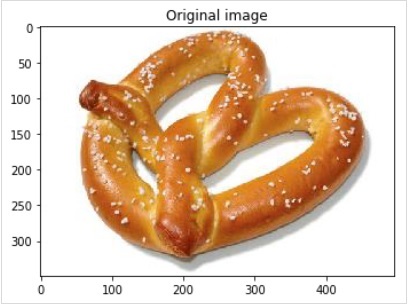
输出如下所示 −
Model predicts pretzel with 0.99999976 confidence
如您所见,预训练模型能够以很高的准确度检测给定图像中的物体。
完整源代码
此处提到了上述代码的完整源代码,该代码使用预训练模型在给定图像中进行物体检测,供您参考 快速参考 −
def crop_image(img,cropx,cropy):
   y,x,c = img.shape
   startx = x//2-(cropx//2)
   starty = y//2-(cropy//2)
   return img[starty:starty+cropy,startx:startx+cropx]
img = skimage.img_as_float(skimage.io.imread("images/pretzel.jpg")).astype(np.float32)
print("Original Image Shape: " , img.shape)
pyplot.figure()
pyplot.imshow(img)
pyplot.title('Original image')
img = resize(img, INPUT_IMAGE_SIZE, INPUT_IMAGE_SIZE)
print("Image Shape after resizing: " , img.shape)
pyplot.figure()
pyplot.imshow(img)
pyplot.title('Resized image')
img = crop_image(img, INPUT_IMAGE_SIZE, INPUT_IMAGE_SIZE)
print("Image Shape after cropping: " , img.shape)
pyplot.figure()
pyplot.imshow(img)
pyplot.title('Center Cropped')
img = img.swapaxes(1, 2).swapaxes(0, 1)
print("CHW Image Shape: " , img.shape)
pyplot.figure()
for i in range(3):
pyplot.subplot(1, 3, i+1)
pyplot.imshow(img[i])
pyplot.axis('off')
pyplot.title('RGB channel %d' % (i+1))
# convert RGB --> BGR
img = img[(2, 1, 0), :, :]
# remove mean
img = img * 255 - mean
# add batch size axis
img = img[np.newaxis, :, :, :].astype(np.float32)
CAFFE_MODELS = os.path.expanduser("/anaconda3/lib/python3.7/site-packages/caffe2/python/models")
INIT_NET = os.path.join(CAFFE_MODELS, 'squeezenet', 'init_net.pb')
PREDICT_NET = os.path.join(CAFFE_MODELS, 'squeezenet', 'predict_net.pb')
print(INIT_NET)
print(PREDICT_NET)
with open(INIT_NET, "rb") as f:
   init_net = f.read()
with open(PREDICT_NET, "rb") as f:
   predict_net = f.read()
p = workspace.Predictor(init_net, predict_net)
results = p.run({'data': img})
results = np.asarray(results)
print("results shape: ", results.shape)
preds = np.squeeze(results)
curr_pred, curr_conf = max(enumerate(preds), key=operator.itemgetter(1))
print("Prediction: ", curr_pred)
print("Confidence: ", curr_conf)
codes = "https://gist.githubusercontent.com/aaronmarkham/cd3a6b6ac071eca6f7b4a6e40e6038aa/raw/9edb4038a37da6b5a44c3b5bc52e448ff09bfe5b/alexnet_codes"
response = urllib2.urlopen(codes)
for line in response:
   mystring = line.decode('ascii')
   code, result = mystring.partition(":")[::2]
   code = code.strip()
   result = result.replace("'", "")
   if (code == str(curr_pred)):
      name = result.split(",")[0][1:]
      print("Model predicts", name, "with", curr_conf, "confidence")
到目前为止,您已经知道如何使用预先训练的模型对数据集进行预测。
接下来是学习如何在 Caffe2 中定义您的 神经网络 (NN) 架构并在数据集上训练它们。我们现在将学习如何创建一个简单的单层 NN。