使用 PyTorch 进行线性回归?
numpypythonpytorch
关于线性回归
简单线性回归基础
让我们了解两个连续变量之间的关系。
示例 −
x = 独立变量
体重
y = 因变量
身高
y = αx + β
让我们通过程序了解简单线性回归−
#简单线性回归

import numpy as np
import matplotlib.pyplot as plt

np.random.seed(1)
n = 70
x = np.random.randn(n)
y = x * np.random.randn(n)

colors = np.random.rand(n)
plt.plot(np.unique(x), np.poly1d(np.polyfit(x, y, 1))(np.unique(x)))

plt.scatter(x, y, c = colors, alpha = 0.5)
plt.show()
输出
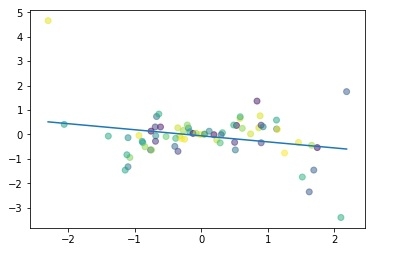
线性回归的目的:
最小化点与线之间的距离 (y = αx + β)
调整
系数:α
截距/偏差:β
使用 PyTorch 构建线性回归模型
假设我们的系数 (α) 为 2,截距(β) 为 1,则我们的方程将变为 −
y = 2x +1 #线性模型
构建数据集
x_values = [i for i in range(11)]
x_values
输出
[0, 1, 2, 3, 4, 5, 6, 7, 8, 9, 10]
#转换为 numpy
x_train = np.array(x_values, dtype = np.float32)
x_train.shape
输出
(11,)
#重要:需要 2D
x_train = x_train.reshape(-1, 1)
x_train.shape
输出
(11, 1)
y_values = [2*i + 1 for i in x_values]
y_values
输出
[1, 3, 5, 7, 9, 11, 13, 15, 17, 19, 21]
#list 迭代

y_values = []
for i in x_values:
result = 2*i +1
y_values.append(result)

y_values
输出
[1, 3, 5, 7, 9, 11, 13, 15, 17, 19, 21]
y_train = np.array(y_values, dtype = np.float32)
y_train.shape
输出
(11,)
#需要 2D
y_train = y_train.reshape(-1, 1)
y_train.shape
输出
(11, 1)
构建模型
#导入库
import torch
import torch.nn as nn
from torch.autograd import Variable

#创建模型类
class LinearRegModel(nn.Module):
def __init__(self, input_size, output_size):
super(LinearRegModel, self).__init__()
self.linear = nn.Linear(input_dim, output_dim)

def forward(self, x):
out = self.linear(x)
return out

input_dim = 1
output_dim = 1

model = LinearRegModel(input_dim, output_dim)

criterion = nn.MSELoss()

learning_rate = 0.01
optimizer = torch.optim.SGD(model.parameters(), lr = learning_rate)

epochs = 100
for epoch in range(epochs):
epoch += 1
#将 numpy 数组转换为 torch 变量
inputs = Variable(torch.from_numpy(x_train))
labels = Variable(torch.from_numpy(y_train))

#清除相对于参数的梯度
optimizer.zero_grad()

#向前获取输出
outputs = model.forward(inputs)

#计算损失
loss = criterion(outputs, labels)

#获取相对于参数的梯度参数
loss.backward()

#更新参数
optimizer.step()

print('epoch {}, loss {}'.format(epoch, loss.data[0]))
输出
epoch 1, loss 276.7417907714844
epoch 2, loss 22.601360321044922
epoch 3, loss 1.8716105222702026
epoch 4, loss 0.18043726682662964
epoch 5, loss 0.04218350350856781
epoch 6, loss 0.03060017339885235
epoch 7, loss 0.02935197949409485
epoch 8, loss 0.02895027957856655
epoch 9, loss 0.028620922937989235
epoch 10, loss 0.02830091118812561
......
......
epoch 94, loss 0.011018744669854641
epoch 95, loss 0.010895680636167526
epoch 96, loss 0.010774039663374424
epoch 97, loss 0.010653747245669365
epoch 98, loss 0.010534750297665596
epoch 99, loss 0.010417098179459572
epoch 100, loss 0.010300817899405956
因此,我们可以将损失从第 1 个时期到第 100 个时期大大减少。
绘制图表
#纯推理
predicted = model(Variable(torch.from_numpy(x_train))).data.numpy()
predicted
y_train

#绘制图表

#清晰图表
plt.clf()

#获取预测
predicted = model(Variable(torch.from_numpy(x_train))).data.numpy()

#绘制真实数据
plt.plot(x_train, y_train, 'go', label ='True data', alpha = 0.5)

#绘制预测
plt.plot(x_train, predicted, '--', label='Predictions', alpha = 0.5)

#图例和图表
plt.legend(loc = 'best')
plt.show()
输出
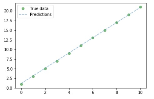
因此,我们可以从图中看出,我们的真实值和预测值几乎相似。